Your Best Feature Might Be Your Biggest Liability

Pre-deployment stability analysis for credit risk models. Catching what IV, CSI, and correlation screening miss.

Jordan Browne-Moore · April 2026

Dataset: Lending Club Accepted Loans (2007-2018) | 30,000 samples | 57 features | 19.78% default rate

The Problem

A feature clears every standard check during development. IV above threshold, correlation structure intact, distribution clean. Then the population shifts slightly and the feature quietly fails in production. Monitoring eventually catches the degradation, but by then the damage is already in the loan book.

I watched this happen repeatedly over nearly half a decade building credit models at Kuda, a Nigerian neobank. Two features stand out in memory. Spend velocity, measuring how quickly money left an account after being deposited, would pass IV screening cleanly but flip its relationship with default depending on the mix of salaried versus gig workers in the sample. The distribution looked stable because both subpopulations spent at similar rates. The signal was not stable because the direction of the relationship with default depended on which subpopulation dominated the draw. Out-of-hours transaction patterns (weekend spend, late-night activity) showed the same behavior.

The problem is that standard screening evaluates marginal properties, not structural resilience. IV gives you one number on the full development set. CSI and PSI tell you a distribution moved after the fact. What none of these tools test is whether the feature’s relationship with default risk is structurally real or just an artifact of who happened to be in the data.

This isn’t a theoretical risk. At Kuda, when enough features drifted into instability, we watched first payment default rates move from 21% to 27% within months. The screened population size didn’t change appreciably, which made it worse: the model was still approving at roughly the same rate while the quality of those approvals was quietly degrading. A 6 percentage point swing in first payment default on a book of meaningful size flows directly into higher provisions, tighter liquidity, and potential covenant issues. By the time monitoring flagged the drift, the losses were already booked.

The toolkit I built to identify these silent liabilities treats feature stability as a learning curve, decomposing instability into a volume component (resolves with more data) and a structural floor (does not resolve). Then it cross-references distributional stability against model-decision stability to identify features that standard screening either wrongly kills or wrongly trusts.

Two Kinds of Stability. Inversely Correlated.

I ran this toolkit on 57 engineered features from Lending Club loan data spanning 2007 through 2018. The features cover credit-seeking velocity, utilisation dynamics, payment discipline, account lifecycle, capacity stress, and loan-level risk: inquiry rates, balance concentrations, DTI variants, delinquency histories. The kinds of features a fintech credit team actually builds.

The scatter plot below scores each of the 14 features that survived forward-CV selection on two axes. The horizontal axis measures marginal complexity: how much the feature’s distributional properties fluctuate under bootstrap resampling, calibrated against a permutation null (the instability you’d expect from a feature with no real relationship to the target). The vertical axis measures SHAP complexity: how consistently a gradient-boosted model uses each feature across bootstrap samples.

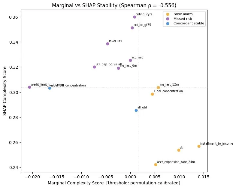
The Spearman rank correlation between the two axes is ρ = -0.556. Not just uncorrelated. Inversely correlated.

Roughly a third of features in this panel do fall into concordant quadrants, meaning the two lenses agree and those features are either confirmed trustworthy or confirmed risky. But for the majority of features, distributional stability and model-decision stability point in opposite directions.

This happens because of collinearity across feature groups. This dataset has nine utilisation features, for instance, each measuring variations of the same underlying behavior. Each individual feature has a clean distribution because the correlated alternatives are distributionally similar. But the model has no reason to prefer one over its near-duplicates. Across bootstrap samples, the model grabs whichever correlated feature happens to be slightly more informative in that draw. The result: individually clean distributions, erratic model usage across the group.

Meanwhile, features like dti and installment_to_income have noisier distributions but carry unique signal that isn’t replicated elsewhere in the feature set. The model has no substitute, so it uses them the same way every time.

Most production feature sets have meaningful collinearity. If yours does, and if you rely on distributional stability as your primary pre-deployment check, you are almost certainly carrying features like the ones this analysis is about to flag.

Two Features. Two Different Decisions.

The metrics below require brief context. Marginal complexity is the weighted structural floor from the learning curve decomposition: negative means the feature stabilizes cleanly, positive means irreducible instability remains regardless of sample size. Direction consistency measures how often the model assigns the same directional effect to the feature across bootstrap samples. SHAP complexity measures the overall instability of the model’s usage of the feature, with lower being more stable.

dti: The wrongly flagged workhorse

Debt-to-income ratio. Marginal complexity of 0.0099 puts it in the upper range, meaning its distributional properties fluctuate meaningfully under resampling. A conservative screening pipeline would flag it for investigation or exclusion.

But the model uses it reliably. Direction consistency of 79.0% places it in the top third of the selected feature set (panel median is 72.4%). SHAP complexity of 0.254 is among the lowest in the panel, meaning the model’s usage of this feature is more stable than most. DTI carries unique information about borrower capacity that isn’t replicated by other features. Standard distributional screening would have penalized a feature the model depends on.

Is 79% direction consistency definitively “stable”? Not in isolation. But relative to a panel where the median is 72.4% and the bottom features sit in the mid-50s, it’s a feature the model uses with meaningfully more consistency than most of its peers. The instability that does exist is concentrated in the distributional noise, not in the model’s usage of the signal.

delinq_2yrs: The silent liability

Number of delinquencies in the past two years. Marginal complexity of 0.0009, near zero. Distributionally, this feature looks rock solid. A standard pipeline would include it without a second thought.

Direction consistency of 55.8%. The model flips the sign of this feature’s effect in nearly half of bootstrap samples. The SHAP complexity of 0.360 is the highest in the entire selected feature set.

A low direction consistency often reveals a feature whose effect is highly conditional on other variables. In a gradient-boosted tree, the delinquency count likely interacts with recency, severity, and account age. In bootstrap samples with different mixes of these interacting features, the net direction shifts. In a scorecard or any model that encodes a fixed coefficient, you cannot represent this conditional relationship. You are forced to average it into a single weight, and averaging an effect that flips sign produces a coefficient near zero: useless at best, misleading at worst.

Beyond scorecard degradation, this directional instability creates a regulatory exposure. If a feature’s effect flips depending on the population segment, using it to generate Adverse Action reasons becomes legally tenuous. The model denies a customer citing delinq_2yrs, but your own bootstrap testing shows the model would have treated that feature as protective in a different segment. That gap is the kind of thing plaintiff’s counsel looks for in a disparate impact case.

The censoring severity of 65.8% compounds the problem. Nearly two-thirds of observations sit at the boundary (zero delinquencies), which creates artificial distributional stability. The feature looks clean because most of its mass is concentrated at a single point. The instability hides in the tail.

How It Works

Instead of computing a single metric on the full development sample, the toolkit constructs an instability curve. It varies pool size from small subsets up to the full dataset, draws multiple bootstrap resamples at each size, and computes distributional metrics (primarily Wasserstein distance and KS statistic) and target-dependent metrics (Spearman correlation, IV) against the full-sample reference. Then it fits k / √n + floor to the resulting curve.

The two parameters tell you different things. k measures how fast instability decays with more data. That’s volume instability, and it resolves with a larger sample. floor measures the irreducible instability that remains even at large n. That’s structural instability, and more data will not help. A positive floor signals that the feature is structurally unstable in its relationship with the target. The confidence interval around the floor estimate can be assessed via meta-bootstrap (repeated stability analysis on different data splits), though the width of that interval depends on dataset size and the number of splits.

Marginal stability and SHAP stability answer different questions and are designed to diverge. Marginal analysis is target-agnostic: it asks whether the feature’s distribution is stable under resampling, and it can run before any model is trained. SHAP analysis is model-dependent: it asks whether the model’s use of the feature is stable across bootstrap samples. Note that SHAP stability inherits the instabilities of whatever model is fitted, so erratic SHAP usage can reflect model sensitivity as well as feature fragility. You need both lenses because, as the Lending Club results show, they can be inversely correlated.

The SHAP stability framework is model-agnostic. This demonstration uses gradient-boosted trees, but the same analysis applies to any estimator that produces feature-level attribution.

How does this compare to existing tools? CSI and PSI detect distributional shift after deployment, but they cannot distinguish structural instability from volume instability before deployment. Out-of-time validation catches temporal drift but requires years of history and confounds time trends with population changes. Bootstrap stability analysis isolates structural fragility from a single snapshot, making it viable for new product launches and thin-history portfolios where temporal holdout data doesn’t exist. Stability selection (Meinshausen & Bühlmann) tests selection probability (binary: does the feature survive regularization?) rather than relationship stability (continuous: in which direction and how consistently does the model use it?). L1/elastic net regularization handles collinearity by penalizing redundant features, but it doesn’t tell you whether the features that survive the penalty have stable relationships with the target or merely stable coefficients in this particular sample. The permutation null calibration in this toolkit gives “unstable” a statistical meaning: it tells you whether the observed instability exceeds what you would expect from a feature with no real relationship to the target.

Source code: github.com/ElSnacko/feature-bootstrapping-toolkit

What the Stability Analysis Actually Produced

Beyond the diagnostic insights, the toolkit drove a concrete feature selection outcome. Starting with 57 engineered features, a forward-CV selection process guided by VIF constraints and incremental AUC lift produced a 14-feature core model. The candidate ordering was by ascending initial VIF (most orthogonal features enter first), making the selection process independent of the marginal stability scores.

AUC dropped from 0.6879 to 0.6631, a loss of 0.025 points on 75% fewer features. Whether that tradeoff is acceptable depends on your monitoring infrastructure costs, data pipeline complexity, and portfolio size. For a lending operation where every additional feature represents a monitoring obligation, a validation documentation burden, and a data pipeline dependency, reducing from 57 to 14 features cuts the ongoing model-risk surface by roughly three-quarters.

The 42 dropped features fell into two categories: 2 were collinear (VIF > 5 without compensating AUC lift) and 40 provided no incremental gain. Many of those 40 were members of large correlated feature groups: exactly the features that showed clean distributions but erratic model usage.

Early Evidence: Structural Floors Predict Temporal Degradation

The Lending Club data spans 2007 through 2018, which allows something the cross-sectional analysis alone cannot: testing whether features flagged as structurally fragile actually degraded in a subsequent time period.

I split the data into a development window (2007–2016) and a holdout window (2017–2018), ran the stability analysis on the development period, and measured how much each feature’s target relationship degraded in the holdout.

Features flagged as structurally unstable in the development period degraded 15x more on average than stable features in the holdout (mean degradation of 1.55 versus 0.10). On the KS metric specifically, the correlation between development-period structural floor and holdout degradation was statistically significant (ρ = 0.727, p = 0.003).

The overall complexity-to-degradation correlation across all metrics is directionally consistent (ρ = 0.332) but not statistically significant at p < 0.05 with only 14 features in the selected set. This is a directional signal, not a predictive guarantee. But the test identified features that did in fact degrade more out of time. That’s the behavior a pre-deployment fragility test is supposed to exhibit.

What This Changes in Your Pipeline

The toolkit produces four concrete integration points in a production credit risk workflow.

1. Pre-model screening. Run marginal stability on all candidate features before training any model. Any feature with a positive structural floor above threshold gets flagged. High censoring severity triggers investigation for upstream truncation, because a feature that looks stable may only look that way because policy rules clipped its tails. On the 30K row Lending Club dataset, the full dual-lens analysis completes in roughly 25 minutes on a 4-core machine. For larger datasets, the permutation null converges quickly, so a stratified 50K-row subsample provides a stable baseline without the full-dataset compute penalty. The marginal metric relies on relative distances rather than absolute population parameters, which is why subsampling preserves the signal.

2. Post-model stability audit. After fitting the model, run SHAP stability on the selected feature set. The “missed risk” quadrant (distributionally clean but model-usage erratic) becomes your second-pass filter. In this dataset, seven features fell into that quadrant, including delinq_2yrs and fico_mid, that would have passed every standard pre-deployment check.

3. Validation documentation. The quadrant classification, floor decomposition, and direction consistency metrics produce a stability report that slots into the SR 11-7 framework for ongoing monitoring and sensitivity analysis. The structural floor is estimated from the development sample; if the production population differs materially, floor estimates should be treated as indicative rather than guaranteed. Detecting material population shift is itself an open problem, which is why this analysis pairs with rather than replaces standard CSI/PSI monitoring.

4. Monitoring integration. The structural floor turns your existing drift alerts into something more actionable. When CSI or PSI triggers on a feature in production, you already know whether the underlying instability is volume-driven (floor near zero, likely a false alarm) or structural (floor is positive, this feature was always fragile, act now). That distinction reduces false alarms and speeds up the retrain-or-intervene decision.

Let’s Talk About Your Features

This framework was built in the context of Nigerian fintech lending, where extreme skew and high default rates make feature stability a first-order concern. The Lending Club demonstration shows the same dynamics emerge in US consumer lending data with standard financial features.

If you’re building or validating credit models and want to stress-test whether your feature set is structurally sound, I run targeted diagnostic engagements where we apply this framework to your data and map the results to actionable model decisions.

Book a call →

The full synthesis report with detailed per-feature results, permutation baselines, and temporal validation outputs is available on request. Source code and documentation at github.com/ElSnacko/feature-bootstrapping-toolkit.